wig

wig has a couple parts. Click the links below or just read through if you’re new here.

MCNP Compilation Help

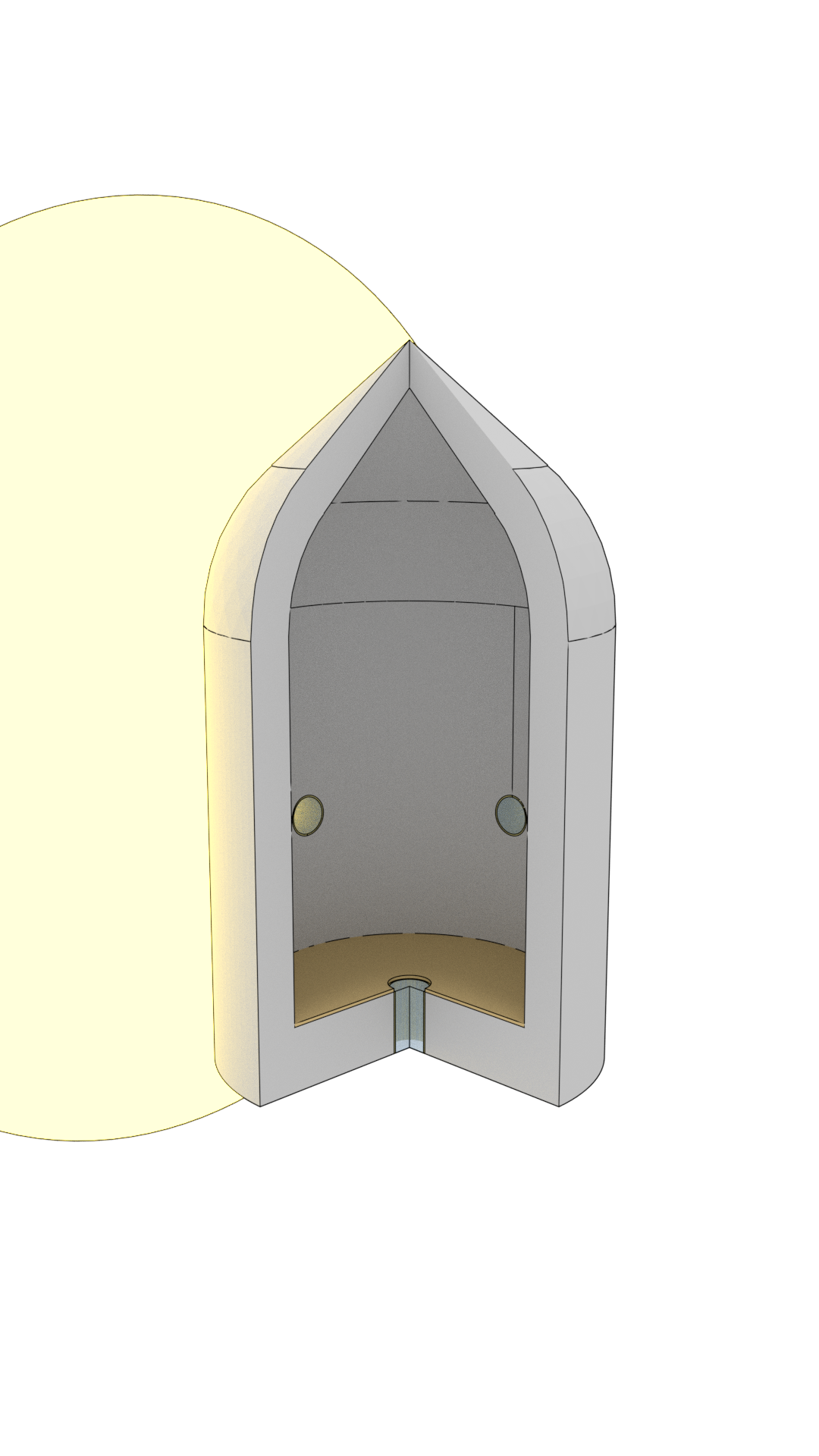
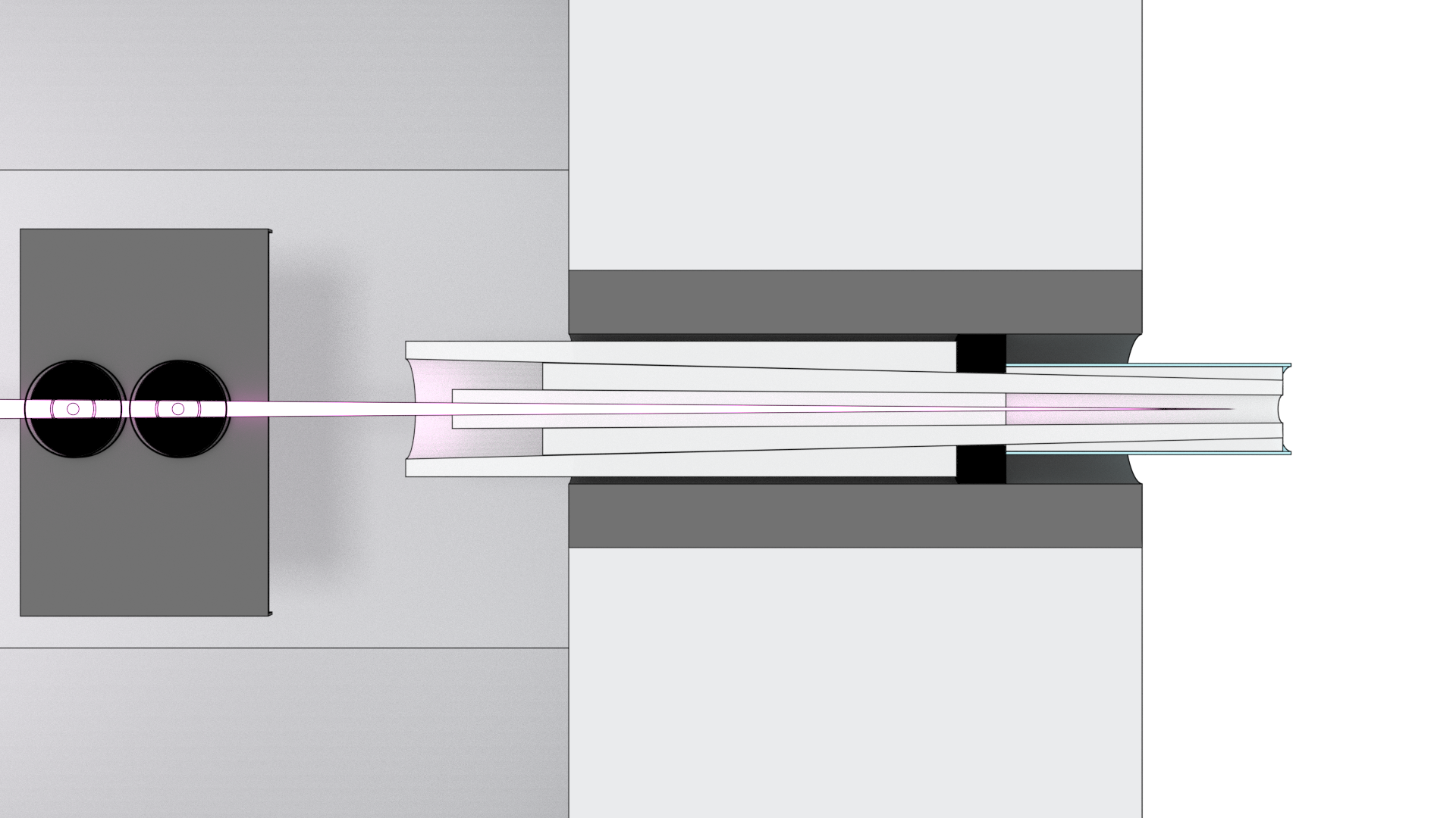
image1 image2 image3

MCNP (Monte Carlo N Particle) software, from LANL, is an incredible tool for simulation of neutrons, photons, and electrons. I use it extensively for my research, and it does a great job at a very complex task. Unfortunately, it’s a nightmare to use. Basically uncompilable by real humans, finicky about input decks and spaces, and almost completely text only (even though Vis-Ed has gotten steadily better), there are lots of improvements that could be made.

I’ll be honest here, I’m writing wig to scratch my own itch. I need a way to:

  • create repeatable input decks
  • automatically create publication worthy figures
  • save geometry and materials as assets somewhere accessible and reusable
  • add some sort of semantic meaning to the syntax of mcnp
  • cite sources in input decks to remember where I got numbers and materials
  • enable easy sending of input decks to be run on “clusters” through ssh

The name is a nod to Eugene Wigner, particularly his contributions to nuclear structure and quantum mechanics, where he made use of the random matrix to describe cross-section structure. MCNP makes use of random numbers to help us experimenters know what’s physically going on, and I want wig to make use of the “random” syntax of MCNP for ease of use. So it’s pronounced vig.

As of now, this package is in a really-really-really alpha stage. I think only I can use it because of it’s finickiness. But, it allows for quick (and semantic) development of MCNP decks using a pipeline method. The pipeline method will be familiar to those that use MCNP a lot. The steps in the pipeline are:

  1. Geometry (create geos)
  2. Materials (create matls)
  3. Cells (combine geos as needed and apply matls)
  4. Physics (there’s a pretty hands off way to define the common physics)
  5. Sources (create source)
  6. Tallies (there’s pretty hands off way for some tally specs now)
  7. Run

The pipeline method means that this package is very semantic, so instead of just typing in numbers separated by spaces, you actually assign variables and document things. You can also script MCNP because of python, for example if you wanted to move a source throughout a bunch of different simulations for time dependence. Finally, this code will, if you have the proper requirements, render pretty pictures of your simulation.

Example - The Moon Voyage

I've waffled on what example to use for wig/MCNP for a while. All the nuclear stuff that isn't boring is, in general, classified or difficult. So, I went for something interesting, but completely unrealistic: Jules Verne's The Moon Voyage. In the book, Mr. Verne describes launching a bullet shaped projectile from Tampa to the moon. I think it'd be interesting to see, among other reasons why the inhabitants would surely be unable to survive, how much radiation dose they would get on their trip. MCNP is great for neutral particles, and not so great for continuum interactions, so we'll ignore the cosmic protons here (which are admittedly a huge part of solar radiation), but we will take into account solar photons with their spectrum.

The first thing we have to do to start the simulation is to import wig. This is reasonably simple: wig has a main class, called wig.wig and then seven other classes, imported below, named (hopefully) self-explanatorially. We should also import numpy, because I can't imagine life without it. And finally, we import some functions that convert imperial units to centimeters, because Mr. Verne didn't know any better than to use them.

In [1]:
from wig import wig, geo, cell, matl, phys, source, tally
import numpy as np
# I know this is bad form, but I want to use feet(9) instead of units.feet(9), it's just easier
from units import *

Now, we'll have to start our scene. We'll use MCNP6 to make use of the new photon libraries (and photoneutron interactions), so to run this, you'll have to have mcnp6 on your path.

In [2]:
scene = wig.wig(filename='moon_voyage_projectile', flavor='6',
                comment='''Solar photons incident on a bullet shaped aluminum
                           projectile from Jules Vernes The Moon Voyage''',
                render=True)

Next, we'll make the geometry. Note that MCNP splits geometry and cells into two modules - you'll have to first define geometries and then combine them into cells. wig attempts to make this more semantic, but it definitely could still use some help. Note also that wig does not have to be written in order. You could write materials, then physics, then sources, then geometry and cells; however, the geometry and materials must be defined before the cells - but that's just basic programming, you have to define variables before you use them.

So below, we'll generate a reasonably complex geometry, as Verne describes the projectile as:

...a cylindro-conical projectile... The projectile outside was nine feet wide and twelve feet high. ...under the wadding were four thick lenticular footlights, two let into the circular wall of the projectile, the third in its lower part...

So now let's get to modeling. First, we need the outer surfaces of the bullet. We'll create a cylinder for the base, a cone for the top, and we'll use a sphere to soften the connection between the cylinder and cone.

In [3]:
# the outside cylinder, centered around the origin - which means the base has to go down halfway
# also, we must convert everything from imperial units to centimeters
# bullet outer radius in centimeters
bullet_or = 4.5 * 12. * 2.540
# bullet cylindrical length in centimeters
bullet_h = 10. * 12. * 2.540
# bullet offset from origin to place the floor at the origin
bullet_dz = -19. * 2.540
# bullet point height is 12 feet, converted to centimeters
bullet_point_z = 16. * 12. * 2.540
bocyl = geo.geo().rcc(c=(0., 0., bullet_dz), r=bullet_or, lz=bullet_h, id='bullet_outer_cyl')
# the sphere to soften the curve - must hit tangent at the top of the cylinder
bosph = geo.geo().sph(c=(0., 0., bullet_dz + bullet_h), r=bullet_or, id='bullet_outer_fillet')
# Now the cone going from a point on the sphere, tangent to the sphere, up to a point
# find the place on the sphere where it is 45deg tangent
dz = bullet_point_z - bullet_h
dz1 = ((dz * dz) - (bullet_or * bullet_or)) / dz
dz2 = dz - dz1
ocone_bottom_h = dz2
ocone_bottom_r = np.sqrt((bullet_or * bullet_or) - (dz2 * dz2))
# Now find the radius at that point
bocone = geo.geo().cone(c=(0., 0., bullet_dz + bullet_h + ocone_bottom_h), r1=ocone_bottom_r, r2=0.1,
                        lz=dz1, id='bullet_outer_point')

Now, we can add the hollow section, which the book claims is 12" thick in most places. We should make the bottom 18" thick, because it was noted to be thicker at the bottom.

In [4]:
bullet_ir = feet(3.5) #3.5 * 12. * 2.540
bullet_ih = feet(8.5) #8.5 * 12. * 2.540
bullet_idz = -inches(1) #-1. * 2.540
bicyl = geo.geo().rcc(c=(0., 0., bullet_idz), r=bullet_ir, lz=bullet_ih, id='bullet_inner_cyl')
# the sphere to soften the curve - must hit tangent at the top of the cylinder
bisph = geo.geo().sph(c=(0., 0., bullet_dz + bullet_h), r=bullet_ir, id='bullet_inner_fillet')
# Now the cone going from a point on the sphere, tangent to the sphere, up to a point
dz = bullet_point_z - bullet_h - feet(1) # (12. * 2.540)
dz1 = ((dz * dz) - (bullet_ir * bullet_ir)) / dz
dz2 = dz - dz1
icone_bottom_h = dz2
icone_bottom_r = np.sqrt((bullet_ir * bullet_ir) - (dz2 * dz2))
bicone = geo.geo().cone(c=(0., 0., bullet_idz + bullet_ih + icone_bottom_h), r1=icone_bottom_r, r2=0.1,
                        lz=dz1, id='bullet_inner_point')

There were at least three portholes, each with a brass surround and glass.

In [5]:
phole1 = geo.geo().rcc(c=(0., 0., - inches(19)), r=inches(5.5), lz=inches(20), id='porthole1')
pholebrass1 = geo.geo().rcc(c=(0., 0., - inches(19)), r=inches(6), lz=inches(20),
                            id='portholebrass1')
phole2 = geo.geo().rcc(c=(-feet(4.5), 0., inches(40)), r=inches(5.5), lx=feet(4.5), id='porthole2')
pholebrass2 = geo.geo().rcc(c=(-feet(4.5), 0., inches(40)), r=inches(6), lx=feet(4.5),
                            id='portholebrass2')
phole3 = geo.geo().rcc(c=(0., -feet(4.5), inches(40)), r=inches(5.5), ly=feet(4.5), id='porthole3')
pholebrass3 = geo.geo().rcc(c=(0., -feet(4.5), inches(40)), r=inches(6), ly=feet(4.5),
                            id='portholebrass3')

The book states that there is a plank of wood holding the room which the inhabitants live in. This is hermetically sealed around the bottom of the inside of the cylinder.

In [6]:
woodcyl = geo.geo().rcc(c=(0., 0., -inches(1)), r=bullet_ir, lz=inches(1), id='wood_disk')

Now that we have those, we can add an enclosing universe, and add all the geometry to the model

In [7]:
uni = geo.geo().sph(c=(0., 0., 0.), r=feet(15), id='universe')
scene.geo([bocyl, bosph, bocone, bicyl, bisph, bicone,
           woodcyl,
           phole1, phole2, phole3,
           pholebrass1, pholebrass2, pholebrass3,
           uni])

Next, we need to define some materials for this model. All of these come from the PNNL Compendium.

In [8]:
# air for the insides of the cabin
air = matl.matl(rho=0.001205, id='air', mass_perc = [('C', 0.000124), ('N-14', 0.755268), ('O-16', 0.231781),
                                                     ('Ar', 0.012827)])
# aluminum - note that aluminum alloys were terrible in Jules Verne's time, so I'll just
# assume that its pure
aluminum = matl.matl(rho=2.6989, id='aluminum', color='#888888', atom_perc = [('Al-27', 1.0)])
# The only wood that PNNL gives us is southern pine - but the book is set in Florida,
# which is pretty southern, I guess
wood = matl.matl(rho=0.640, id='wood', color='#966F33',
                 atom_perc = [('H-1', 0.462423), ('C', 0.323389), ('N-14', 0.002773),
                              ('O-16', 0.208779), ('Mg', 0.000639), ('S', 0.001211),
                              ('K', 0.000397), ('Ca', 0.000388)])
# Plate glass for the windows - who knows if they can be casted that thick
glass = matl.matl(rho=2.4, id='glass', color='#7299c6', alpha=0.4,
                  atom_perc = [('O-16', 0.603858), ('Na-23', 0.088145), ('Si', 0.251791),
                               ('Ca', 0.056205)])
# Brass for the surrounds on the outside of the windows
brass = matl.matl(rho=1.0, id='brass', color='#b5a642',
                  atom_perc=[('Fe', 0.001002), ('Cu', 0.674918), ('Zn', 0.320956),
                             ('Sn', 0.001451), ('Pb', 0.001673)])
void = matl.matl(rho=0.0, id='void', mass_perc = [])
scene.matl([air, aluminum, wood, glass, brass])

Now, to make the cells using the geometry and the materials.

In [9]:
%%capture
bullet_cell = cell.cell(bocyl + bosph + bocone - bicyl - bisph - bicone - 
                        pholebrass1 - pholebrass2 - pholebrass3, aluminum)
wood_cell = cell.cell(woodcyl - pholebrass1, wood)
window_1_b = cell.cell(pholebrass1 - phole1 - bicyl, brass)
window_1 = cell.cell(phole1 - bicyl, glass)
window_2_b = cell.cell(pholebrass2 - phole2 - bicyl, brass)
window_2 = cell.cell(phole2 - bicyl, glass)
window_3_b = cell.cell(pholebrass3 - phole3 - bicyl, brass)
window_3 = cell.cell(phole3 - bicyl, glass)
air_cell = cell.cell(bicyl + bisph + bicone - woodcyl, air, show=False)
uni_cell = cell.cell(uni - bocyl - bosph - bocone, void, show=False)
scene.cell([bullet_cell, wood_cell,
            window_1, window_2, window_3,
            window_1_b, window_2_b, window_3_b,
            air_cell, uni_cell])

Now that we have the geometry built, we need some details about the physics. We're only going to take into account photons for now, and their energies need to span a huge range - we'll span the entire range of the solar irradiance dataset from Wehrli 1985, which is $199.5\mathrm{nm}$ to $10075.0\mathrm{nm}$ (or $.123\mathrm{eV}$ to $6.2\mathrm{eV}$).

In [10]:
# Add some typical neutron physics
physics = phys.phys(particles='p', nps=1E8, maxE=6.2E-6, minE=0.123E-6)
scene.phys(physics)

Now, we'll add a source. The projectile is far enough from the sun to assume that the sun is a plane source. We'll add a source covering the projectile to the $-x$ direction in our model. The spectrum is taken from the ASTM E490-0 AM0 old Spectrum from NREL and Wehrli. I've downloaded a text file from NREL and will use it to plot the spectrum below. Then, we'll have to convert this to flux instead of irradiance using the formula $$F\left(\lambda\right) = \Phi E \frac{1}{\Delta \lambda}$$ and by solving for $\Phi$ $$\Phi = F\left(\lambda\right)\frac{\Delta\lambda}{E}$$ We're using a couple libraries I maintain for data analysis and plotting called pym and pyg, respectively.

In [11]:
from pym import func as pym
from pyg import twod as pyg2d
import shutil
# Wehrli gives irradiance in W/m^2/nm
wavelength, irradiance, _ = \
    np.loadtxt(scene.original_directory + '/wehrli85.txt', unpack=True, skiprows=2)
h = 4.135668E-15 # planck's constant in eV s
c = 2.998E+17 #speed of light in nm/s
E = h * (c / np.array(wavelength))
# Conversion to flux (and converting eV to J)
Phi = (irradiance / (E * 1.6E-19)) * wavelength
flux_spectrum = pym.curve(E, Phi, name='solar_flux_spectrum')
plot = flux_spectrum.plot(linestyle='-')
plot.xlabel(r'Photon Energy ($E$) [$\mathrm{eV}$]')
plot.ylabel(r'Flux ($\Phi$) [$\mathrm{\frac{\text{photon}}{m^{2} \cdot s}}$]')
plot.markers_off()
plot.export('solar_spectrum', ratio='silver')
shutil.copy('solar_spectrum.svg', scene.original_directory + '/solar_spectrum.svg')
plot.show('The solar spectrum from Wehrli 1985 in energy units', label='solspec')
Figure 1: The solar spectrum from Wehrli 1985 in energy units
In [12]:
# add the source
sun = source.source(particle='p', pos=(0., -feet(8), feet(6)), id='sun',
                    shape='disk', direction='+y', radius=feet(12), 
                    spectrum=[E, Phi])
scene.source([sun])

And let's check a tally or two. I think we'd like to have a flux tally inside of the chamber, and also a heating tally in the bullet cell. These commands should be pretty semantic

In [13]:
# add some tallys
mesh_tally = tally.tally(comment='compartment_mesh', particle='p')\
    .mesh_tally(xmin=-feet(4.5), xmax=feet(4.5), i=9*12,
                ymin=-feet(4.5), ymax=feet(4.5), j=9*12,
                zmin=0.0, zmax=feet(10), k=10*12)
energy_tally = tally.tally(comment='aluminum_heating', particle='p', energy=[0.123E-6, 6.2E-6])\
    .energy_tally(tally_cell=bullet_cell)

scene.tally([energy_tally, mesh_tally])

Now, we can run it. We want to do a rendering of the geometry, so we'll look at that first.

In [14]:
scene2 = scene.bscene
scene2.cutaway(c=(100., 100., feet(8)), l=(200., 200., feet(20)))
scene2.run(res=[1080, 1920], samples=100, 
           c=(0., 0., feet(6)), camera_location=(700., 700., 375.))
In [15]:
from pyg import three2twod as pyg32d

shutil.copy('brender_01.png', scene.original_directory + '/moon_voyage.png')
plot = pyg32d.ann_im(scene.original_directory + '/moon_voyage.png')
plot.add_data_pointer(0., -feet(8), feet(6) + feet(12),
                      string=r'Sun (disk photon source)',
                      place=(-200., 200.))
plot.add_legend_entry(color='#888888', name='Aluminum')\
    .add_legend_entry(color='#b5a642', name='Brass')\
    .add_legend_entry(color='#7299c6', alpha=0.4, name='Glass')\
    .add_legend_entry(color='#966F33', name='Wood')
plot.legend(loc=2)
plot.export('moon_voyage', force=True, ratio='invgolden')
shutil.copy('moon_voyage.svg', scene.original_directory + '/moon_voyage.svg')
plot.show('Depiction of the Moon Voyage\'s cylindo-conical projectile',
          label='moonvoyageprojectile')
Figure 2: Depiction of the Moon Voyage's cylindo-conical projectile

And finally, we can run it. I'll check back in in a week or so with the results!

In [16]:
%%capture
#scene.run(render=False)

Main object

wig.wig object

class wig.wig.wig(comment, filename, flavor=‘6’, render=True, particles=[‘n’])[source]

The wig object is the base object for an MCNP setup.

The wig object is basically the scene in which we create our MCNP geometry, cells, materials, physics, tallies, and other data. I usually just call it scene and use it from there.

Parameters:
  • comment (str) – The comment that will be placed BELOW the first comment line of the MCNP deck.
  • filename (str) – The filename (duh) of the input deck. ‘.inp’ will be automatically appended. The full path to this file will be the first line of the input file (i.e., the full path will be the first comment line of the deck)
  • flavor (str) – ‘6’ for mcnp6, ‘5’ for mcnp5, ‘x’ for mcnpx, or ‘polimi’ for mcnpx-polimi. Make sure you alias the binaries to those commands or the runner wont work.
  • render (bool) – defines whether to render the scene using blender before running it
  • particles (list) – a list of 'n', 'p', ... for the particles we should care about
Returns:

the wig object.

set_filename(filename)[source]

set_filename sets the base of the filenames that will be created

Parameters:filename (str) – the base of the filename
set_comment(comment)[source]

set_comment writes the first line of the mcnp file, which is a comment describing the file. Be descriptive but not too long.

Parameters:comment (str) – the first line of the mcnp file - limit is 80 characters. wig manually strips newlines, so feel free to make this a triple quoted (''') string with as many returns as you like.
geo(geos=None)[source]

geo adds all defined wig.geo objects to an input deck

Parameters:geos (list) – the wig.geo objects to be added to the input deck. Make sure this includes a universe
add_geo(geos=None)[source]
redefine(name=None)[source]
cell(cells=None, auto_universe=True, universe_matl=None, debug_blender=False)[source]

cell adds all the wig.cell in a list to an input deck.

Parameters:
  • cells (list) – the list of wig.cell to be added to the input deck. If you don’t have a cell named 'universe', this method will make one for you, but you might night like it.
  • debug_blender (bool) – whether or not you want to see the commands that will be sent to blender, default False.
make_universe(geo=None, matl=None)[source]
matl(matls=None)[source]

matl adds all the wig.matl to the input deck

Parameters:matls (list) – the materials to add to the input deck
add_matl(matls=None)[source]
phys(phys=None)[source]

phys adds all wig.phys blocks to the model

Parameters:phys (wig.phys) – the wig.phys block to be added to the model.
tally(tallies=None)[source]

tally adds all wig.tally b’ocks to the model

Parameters:tallies (list) – the wig.tally blocks to be added to the model.
source(sources=None)[source]

source adds the wig.source object to the model

Parameters:sources (list) – the wig.source blocks (defining sources and distributions) to be added to the model.
run(remote=’local’, sys=’linux’, blocking=False, clean=False, **kwargs)[source]

run (of course) runs the deck.

run first writes the input deck, including rendering with whatever additional keyword args you pass, and then opens an instance of a wig.runner , and passes commands to it.

Parameters:
  • remote (str) – The ip address of the remote system you want to run this on, or 'local' if on this system. The remote system must be set for passwordless ssh login and have mcnp on path (whatever flavor you’re using). Default: 'local'
  • sys (str) – The type of system that the remote runs on. Currently, this is useless, as I’ve only made it run on linux. Default: 'linux'
  • blocking (bool) – Whether to wait on the deck to finish running before continuing or not. Useful to block if you want to run many decks depending on the previous result (optimization), or if you only have a certain number of processors. Default: False
  • clean (bool) – Whether to clean up the running files in the ~/mcnp/active directory or not. Keep the files if storage isn’t a concern and you’re unsure if your deck will run correctly. Default: False
  • kwargs (dict) – run passes the rest of the commands to write
write(**kwargs)[source]

write writes the input deck and renders the input deck

Parameters:kwargs (dict) – keyword arguments to pass to render
render(filename_suffix=”, render_target=None, camera_location=None, render=True, **kwargs)[source]

render passes the input deck to pyb, a simplified renderer that uses blender as the backend

Parameters:
  • filename_suffix (str) – suffix to put after the filename when we save the rendering. Default: ''
  • render_target (tuple) – a point for the camera to look at when rendering. Default: (0, 0, 0)
  • camera_location (tuple) – a point from which the camera looks. Default: based on the size of the scene, isotropic placement.
  • render (bool) – Whether or not to actually run the render. This method will always save a blender file, regardless of if we do a full render. Default: True
  • kwargs (dict) – Other arguments to pass to pyb.render. See pyb for options, such as samples or res.
refresh_data()[source]

refresh_data resets the data block to nothing. Useful if you’re reusing a model and want to reset sources or materials or something.

refresh_geo()[source]

refresh_geo resets the geometry block to nothing. Useful if you’re changing geometry, although this probably shouldn’t be used without also refreshing the cells. But I don’t know you, live your life.

refresh_cell()[source]

refresh_cell resets the cell block to nothing. Again, useful for changing up cell definitions or materials.

refresh_phys()[source]

refresh_phys resets the physics block to nothing. This is a subset of the refresh_data method, so use whichever one is more useful.

refresh_source()[source]

refresh_source resets the soruce block to nothing. This actually just calls refresh_data because the only thing in the data block right now is the sources.

refresh_tally()[source]

refresh_tally resets the tally block to nothing. This is probably not useful, unless you’re changing other things, too. If the model is still the name, just add the all the tallies in one input file and run it, it’s faster that way.
refresh_matl()[source]

refresh_matl resets the materials block to nothing. Super useful if you’re messing around with shielding, or reactions.

go_home()[source]

wig runs in the directory ~/mcnp/active. go_home goes to the directory in which the script started.

Input Deck Creation Submodules

wig.geo object

class wig.geo.geo[source]

a wig.geo instance is a single geometric primative for creation of the geometry block for MCNP. Where possible, I’ve used macrobodies instead of surfaces; this decision may be problematic for purists, but surfaces are so convoluted to use.

boolean(right, operation)[source]

wig.geo implements some of the boolean geometry used by MCNP. The operators usable are:

  • + - implements a geometric boolean union operator between the two objects
  • - - implements a geometric boolean difference operator between the two objects
  • | - implements a geometric boolean union operator between the two objects
  • % - implements a geometric boolean intersection operator between the two objects

For example, the following creates a cube on a stick

1
2
3
4
cube = wig.geo().rpp(x=[0., 5.], y=[0., 5.], z=[0., 5.], id='1')
stick = wig.geo().rcc(c=(2.5, 2.5, -5.), r=1., lz=5., id='2')
cube_on_a_stick = cube + stick
cube_on_a_stick_cell = cube_on_a_stick.cell(some_material)

Todo

Implement more boolean operators

rpp(c=None, l=None, x=None, y=None, z=None, id=None)[source]

rpp is the same as the MCNP macrobody, a right parallelpiped.

rpp has two ways to define it:

  • center (c) and length (l)
  • \(x\) extents (x), \(y\) extents (y) and \(z\) extents (z)
Parameters:
  • c (tuple) – the center of the right parallelpiped
  • l (tuple) – the length of each side, centered at c
  • x (list) – the \(x\) extents of the right parallelpiped, always with the lowest number first.
  • y (list) – the \(y\) extents of the right parallelpiped, always with the lowest number first.
  • z (list) – the \(z\) extents of the right parallelpiped, always with the lowest number first.
  • id (str) – an identifying string with no spaces
box(v=None, a1=None, a2=None, a3=None, id=None)[source]

box is similar to rpp, but is not oriented to the cartesian axes. Instead, you must define three axes, which are orthagonal to each other, as well as the corner (v).

Parameters:
  • v (tuple) – The corner of the box
  • a1 (tuple) – the vector defining one edge emanating from v
  • a2 (tuple) – the vector defining one edge emanating from v
  • a3 (tuple) – the vector defining one edge emanating from v
  • id (str) – an identifying string with no spaces

Todo

calculate the a3 from a1 and a2, if given

Todo

calculate the box from three points

sph(c=None, r=None, id=None)[source]

sph defines a sphere with radius r at c

Parameters:
  • c (tuple) – the center of the sphere
  • r (float) – the radius of the sphere
  • id (str) – an identifying string with no spaces
rcc(c=None, r=None, id=None, lx=None, ly=None, lz=None)[source]

rcc defines a right circular cylinder. The geometry can be specified by defining the center of the base c, radius r, and one of lx, ly, or lz which is the height in one of those ordinal directions.

Parameters:
  • c (tuple) – center of the base of the cylinder
  • r (float) – radius of the circular base
  • lx, ly, lz (float) – height in one of the ordinal directions
  • id (str) – an identifying string with no spaces

Todo

allow a vector l to define slanted cylinders

gq(A=None, B=None, C=None, D=None, E=None, F=None, G=None, H=None, J=None, K=None, coeffs=None, id=’gq’)[source]
gq` creates a generalized quadratic surface defined by the

equation

Warning

This is not implemented as of yet. Just a placeholder.

\[\begin{split}Ax^{2}+By^{2}+Cz^{2}+Dxy+Eyz\\+Fzx+Gx+Hy+Jz+K=0\end{split}\]

and takes inputs of either \(A\), \(B\), \(C\), \(D\), \(E\), \(F\), \(G\), \(H\), \(J\), \(K\), or an array coeffs which has the coefficients (all 10 of them) defined in alphabetical order.

Parameters:
  • A (float) – the coefficient \(A\)
  • B (float) – the coefficient \(B\)
  • C (float) – the coefficient \(C\)
  • D (float) – the coefficient \(D\)
  • E (float) – the coefficient \(E\)
  • F (float) – the coefficient \(F\)
  • G (float) – the coefficient \(G\)
  • H (float) – the coefficient \(H\)
  • J (float) – the coefficient \(J\)
  • K (float) – the coefficient \(K\)
  • coeffs (list) – a (10,) or (1,10) size array containing the coefficients \(A\) through \(K\), respectively
Returns:

the generalized quadratic surface object

Todo

Implement the gq surface

cone(c=None, dir=’+z’, h=None, r=None, r1=0.0, r2=0.0, lx=0.0, ly=0.0, lz=0.0, id=0.0)[source]

cone makes a truncated cone. It allows for specifications of the cone in two ways:

  • base center c, radii r1 and r2, height h in direction dir
  • base center c, radii r1 and r2, height lx, ly, or lz in the implied direction
Parameters:
  • c (tuple) – the base center of the cone
  • dir (str) – one of +x, -x, +y, -y, +z, -z
  • h (float) – height of the cone
  • r1 (float) – base radius
  • r2 (float) – top radius
  • r (list) – size two list of base and top radius, respectively
  • lx, ly, lz (float) – height in respective direction
  • id (str) – an identifying string with no spaces
cell(matl)[source]

geo.cell(matl) returns a cell of this geometry with material matl

Parameters:matl (wig.matl.matl) – The material to make this cell
Returns:mcnpce.cell object

wig.matl object

class wig.matl.matl(rho, atom_perc=None, mass_perc=None, id=None, color=None, alpha=1.0)[source]

matl defines a material for the MCNP format with definitions in either mass or atom percent. The list passed to atom_perc or mass_perc is formatted as:

steel_atom_perc = [('C-12', 0.022831), ('Fe', 0.995000)]

note that the isotope convention 'C-12' evaluates to ZAID 006012 and the element convention 'Fe' just evaluates to ZAID 026000.

Parameters:
  • rho (float) – the density of the material in \(\frac{g}{cm^{3}}\)
  • atom_perc (list) – list formatted as above of atom percentages
  • mass_perc (list) – list formatted as above of mass percentages
  • id (str) – an identifying string with no spaces
  • color (str) – the color of the material for rendering, in hex format '#RRGGBB'
  • alpha (float) – the opacity of the material for rendering, from 0.0 to 1.0. Default: 1.0

Todo

define an asset based materials import system

wig.cell object

class wig.cell.cell(geo=None, matl=None, comment=None, color=None, alpha=1.0, show=True)[source]

a cell is a combination of geometric primitives (single or combined using geo operators) and the material applied to that section of geometry. The easiest way to get a cell is to simply call geo().cell(matl) on the geometry object, but for more explicit uses, instantiation of this class can be useful.

Parameters:
  • geo (wig.geo) – the geometry object, whether singular or combined
  • matl (wig.matl) – the material object
  • comment (str) – a comment that will be printed beside the cell
  • show (bool) – whether or not the object will be shown in the rendering
  • color (str) – the color for the material in the rendering, in hex format (‘#RRGGBB’)
  • alpha (float) – the opacity of the object in the rendering, from 0.0 to 1.0, Default: 1.0
static air()[source]

air is the common material for the universe.

air is a static method that returns the PNNL compendium defined air material for use as universe materials, or others. It should be decided whether to use this class or the materials class as a repository for materials.

Todo

define an assets system for this.

refresh()[source]

refresh removes all of the blender commands from the cell. Useful for if you are changing cells with new geometry or color.

wig.phys object

class wig.phys.phys(particles=None, sources=None, maxE=None, minE=None, nps=None, ctme=None, polimi=False, polimi_cells=[], ipol=[0, 0, 0], rpol=[0, 0, 0])[source]

phys defines all of the options for physics in the MCNP model

Parameters:
  • particles (list) – list of particles included, such as ['p', 'n']
  • sources (list) – Not implemented
  • maxE (float) – maximum energy (in \(MeV\)) to model
  • minE (float) – minimum energy (in \(MeV\)) to model
  • nps (int) – number of particles to simulate
  • ctme (int) – number of minutes to run the model
  • polimi (bool) – whether this is an MCNP-Polimi deck. Do not use when not using wig.flavor = 'polimi'.
  • polimi_cells (list) – cells in which to transport neutrons/photos using MCNP-Polimi
nps(num)[source]

nps is a convenience method to change the number of particles to simulate

Parameters:num (int) – number of particles, maximum around 2E9 unless you’ve compiled MCNP with 64-bit integers
ctme(num)[source]

ctme is a convenience method to change the number of minutes to run the deck.

Parameters:num (int) – number of minutes to run. Beware that if the number of particles exceeds the maximum integer, the simulation will fail.
no_fission(cells=None)[source]

no_fission removes creation of neutrons from fission in certain cells using MCNP’s nonu directive.

Parameters:cells (list) – list of cell in which to remove fission
polimi(cells=[], out_src=False)[source]

polimi is a convenience method to use MCNP-Polimi to transport particles through the cells in cells.

Parameters:
  • cells (list) – list of cell to use MCNP-Polimi for transport
  • out_src (list) – if you want to output the source

wig.source object

class wig.source.source(particle=’n’, pos=None, x=None, y=None, z=None, spectrum=None, shape=None, direction=None, id=None, radius=None, cell=None, show=True, spectrum_type=’C’, axis=None, lx=None, ly=None, lz=None, anisotropic=False)[source]

source is an object that defines an MCNP source. Currently there are only a few implemented type of sources:

  • point source: use pos or x, y, and z
  • disk source: use pos, shape = 'disk', and direction
  • cell source: use cell and an enclosing disk
  • energy spectrum: use spectrum and a dist object
  • intensity distribution:
Parameters:
  • particle (str) – one of ‘n’, ‘p’, ‘d’, ‘t’, ‘s’, ‘a’, or ‘fission’
  • pos (tup) – position of the source
  • x, y, z (float) – position of the source - alternate method
  • spectrum – either a distribution or a two-d list to create an energy distribution
  • shape (str) – right now, can only be 'disk', more coming.
  • direction (str) – one of ‘+x’ or ‘-x’, ‘+y’ or ‘-y’, or ‘+z’ or ‘-z’
  • id (str) – an identifying string
  • radius (float) – the radius of a disk source
  • cell (wig.cell) – the cell for a volumetric source
  • show (bool) – whether the source should be rendered or not

Todo

implement the whole MCNP Primer of sources

wig.tally object

class wig.tally.tally(**kwargs)[source]

a tally object defines one of several types of MCNP tallies:

  • flux tally (f4)
  • current tally (f1)
  • fission tally (f7)
  • mesh tally (fmesh4)

The best pratice is to pass energies and comments to the initializer and to use the convenience methods to continue from there

Es = [1.0E-4, 1.0, 100.0]
meshtal1 = wig.tally(comment='a mesh tally for demo purposes', energy=Es)                .mesh_tally(xmin=0.0, xmax=10.0, ymin=0.0, ymax=10.0, zmin=0.0, zmax=10.0, ijk=(10, 10, 10))
flux_tally(**kwargs)[source]

flux_tally is a tally calculating the flux through a cell. Pass keywords energy, cell, and particle

energy_tally(**kwargs)[source]

energy_tally is a tally calculating the energy deposited in a cell per unit mass.

Parameters:
  • energy (list) – A list whos energies span the range of the highest to lowest interesting energies
  • tally_cell (object) – the cell of interest
  • particle (str) – ‘n’ for neutrons, ‘p’ for photons, or ‘n, p’ for both
rmesh(**kwargs)[source]
mesh_tally(**kwargs)[source]

mesh_tally is a tally finding the mesh in many voxels. Pass keywords xmin, xmax, ymin, ymax, zmin, zmax, and list ijk or i, j, and k, which are the number of voxels in the x, y, and z directions, respectively

add_multiplier(**kwargs)[source]

add_multiplier adds the multiplier defined by mt in keywords on material from keyword mat. You can also add a constant C or leave that to default 1.

current_tally(**kwargs)[source]

current_tally is a tally calculating the current through a surface. Pass keywords energy, surfaces, and particle

fission_tally(**kwargs)[source]

fission_tally is a tally calculating the fissions in a cell. Pass keyword cell.

process_energy(**kwargs)[source]

process_energy prints the energies in keyword energy into MCNP notation

Run and Runtime Submodules

wig.runner object

class wig.runner.runner(filename, command, remote=’local’, sys=’linux’, blocking=False, clean=False, just_write=False, **kwargs)[source]

runner is an object that ssh’s to a remote (or local) system and starts a wig job, assume that it is set up completely and correctly. You can define your systems to run this on in ‘~/.wig/config.py’ as the dict systems with structure

systems = {"tianhe-2": {"ip": "255.255.255.255", "port": 22,
                        "username": "nscwadmin", "password": "123",
                        "procs": 10649600},
           "titan": {"ip": "255.255.255.255", "port": 22,
                     "username": "ornladmin", "password": "123",
                     "procs": 560640},
           "local": {"ip": "", "port": "",
                     "username": "", "password": "",
                     "procs": 4}}

Todo

write article/todo on how to setup this

Parameters:
  • filename (str) – base name of the file to run
  • command (str) – command which will call the desired flavor of MCNP
  • remote (str) – string identifying the remote system
  • sys (str) – type of system this will run on, currently only supported for 'linux', although 'OSX' would probably be easy
  • blocking (bool) – whether to wait for the MCNP run to finish before continuing. Default False.
  • clean (bool) – whether to clean the old files with the same base filename from filename from directory ~/mcnp/active/. Useful if you’ve screwed something up and want to start fresh

wig.mcnpdaemon object

class wig.mcnpdaemon.mcnpdaemon[source]

Todo

Make a daemon to watch this, using Flask

set_notification_daemon(notification)[source]
run()[source]
check_file()[source]

Post-processing Submodules

wig.analyze object

class wig.analyze.analyze(filename, nps=None, tmesh=False)[source]

analyze goes through an output file and checks for tallies.

An analyze object will hold tally objects in a list, one for each of the printed tallies on the file filename, if these were generated as a tally file through mcnp. Tallies printed on the .out file currently do not have support.

Todo

Add support for tallies printed in a .out file.

Parameters:filename (str) – filename of the tallies.out file
import_meshtal_section(section)[source]
import_tmesh_section(section)[source]
import_tally_section(section)[source]

Convenience and internal submodules

wig.mcnp_string object

class wig.mcnp_string.mstring(string)[source]

mstring are strings that can be printed in MCNP files. MCNP is so finicky, and same with Python (with respect to indentation), that it’s easier to just remove all newlines and split everything into 80 character blocks.

Parameters:string (str) – a string, formatted however, that will be converted to MCNP format
flow()[source]

flow actually converts the string to MCNP format.

Return str string:
 a string with newlines in 80 character blocks

Indices and tables

Contents

Tests

Todo

write tests

ToDos

Todo

Implement more boolean operators

(The original entry is located in /home/ahagen/code/wig/geo.py:docstring of wig.geo.geo.boolean, line 19.)

Todo

calculate the a3 from a1 and a2, if given

(The original entry is located in /home/ahagen/code/wig/geo.py:docstring of wig.geo.geo.box, line 11.)

Todo

calculate the box from three points

(The original entry is located in /home/ahagen/code/wig/geo.py:docstring of wig.geo.geo.box, line 13.)

Todo

allow a vector l to define slanted cylinders

(The original entry is located in /home/ahagen/code/wig/geo.py:docstring of wig.geo.geo.rcc, line 11.)

Todo

Implement the gq surface

(The original entry is located in /home/ahagen/code/wig/geo.py:docstring of wig.geo.geo.gq, line 29.)

Todo

define an asset based materials import system

(The original entry is located in /home/ahagen/code/wig/matl.py:docstring of wig.matl.matl, line 21.)

Todo

define an assets system for this.

(The original entry is located in /home/ahagen/code/wig/cell.py:docstring of wig.cell.cell.air, line 8.)

Todo

implement the whole MCNP Primer of sources

(The original entry is located in /home/ahagen/code/wig/source.py:docstring of wig.source.source, line 22.)

Todo

write article/todo on how to setup this

(The original entry is located in /home/ahagen/code/wig/runner.py:docstring of wig.runner.runner, line 18.)

Todo

Make a daemon to watch this, using Flask

(The original entry is located in /home/ahagen/code/wig/mcnpdaemon.py:docstring of wig.mcnpdaemon.mcnpdaemon, line 1.)

Todo

Add support for tallies printed in a .out file.

(The original entry is located in /home/ahagen/code/wig/analyze.py:docstring of wig.analyze.analyze, line 8.)

Todo

write tests

(The original entry is located in /home/ahagen/code/wig/docs/index.rst, line 25.)